![]()
Introduction
🌈 Colorify makes color creation and modification intuitive and effortless. Colorify is lightweight and dependency-free yet combines functionality of popular color and visualization packages, including:
- viridis palettes, that are perceptually uniform and colorblind-friendly: Viridis, Turbo, Inferno, Cividis, Plasma, Rocket & Mako.
- Rcolorbrewer palettes and inspired palette visualization.
- ggplot2 easy-to-use integration of scale_color_* and scale_fill_* bindings.
- base R (grDevices) palettes: Rainbow, Heat, Terrain, Topo, Cm & all hcl/pal palettes.
- Okabe-Ito palette, for a highly distinct and colorblind-safe scheme.
Why use coloRify?
Colorify is dependency-free, yet offers access to all popular palettes and color functionality described above!
If you are, like me, tired of errors complaining you need more colors than your palette contains? No problem! Colorify generates maximally different colors alongside custom palettes based on how many colors are requested.
Colorify enables effortless palette/color modification, based on the intuitive RGB and HSL color spaces.
How coloRify works
See the examples below for the following functionality:
-
colorify(): the main function offers call parameters for most-in-one color/palette creation and modification tools, the other functions are in support of this, as will be shown in the examples and documentation below.
- colorify_pal(): colorify() wrapper to return a color palette generator function
display_palettes(): view coloRify palettes that are used with colorify(colors = …)
ggplot2 bindings: scale_fill_colorify() & scale_color_colorify
utilities for color space conversion: hex2rgba() & hsv2rgb()
colortistry(): #Rtistry creative fun
Examples
To run coloRify, simply install the package from CRAN…
install.packages("colorify")…or the development version from GitHub
pak::pkg_install("colorify", dependencies = TRUE, upgrade = TRUE)Then load the library.
Note that coloRify uses hexcolors (e.g.: “#FF0000FF”) and includes base R colors (e.g.: “red”) from grDevices:
grDevices::colors()colorify()
basic
A basic call with just n(=10) colors requested. n takes an integer > 0.
colorify(n = 10, plot = TRUE)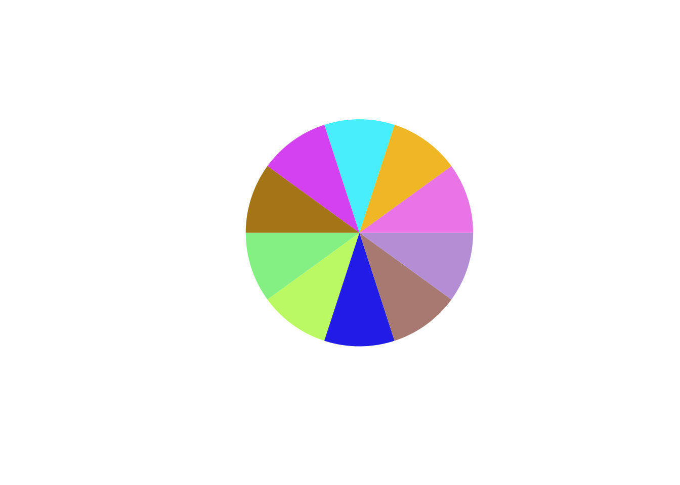
#>  [1] "#E974E6FF" "#EEB723FF" "#48EEFCFF" "#D341F1FF" "#A37515FF" "#84EF83FF"
#>  [7] "#BBF963FF" "#221DE6FF" "#A77971FF" "#B38ED5FF"
See in the output above that coloRify returns a hexcolor vector.
seed
To show that a different seed yields different generated colors. Pass seed as an integer.
c <- colorify(10, plot = TRUE, seed = 1337)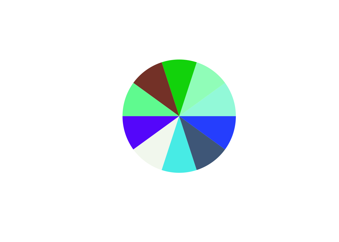
custom colors
You can give custom colors and generate the rest, always have enough colors for plotting calls!

naming
Set names to the output hexcolor vector. colors_names takes a character vector of names the length of the amount of requested colors.
c <- colorify(colors = c("red", "white", "blue"), n = 5, colors_names = paste0("name", rep(1:5)), plot = TRUE)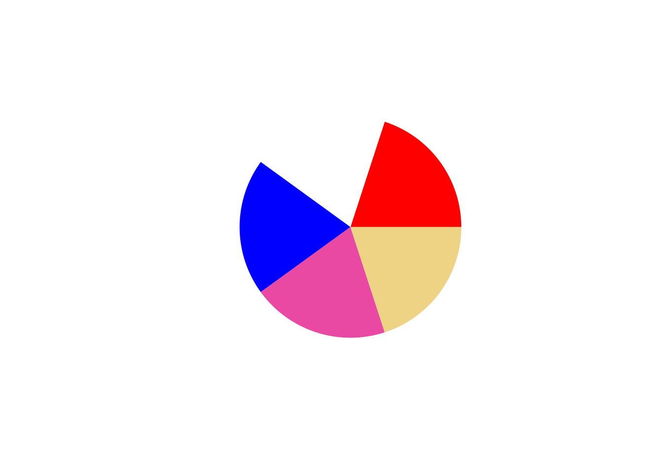
ordering
Order the hexcolor output. Integer given as starting point for ordering, may be negative.
# set integer for the ordering starting position
c <- colorify(colors = c("red", "white", "blue"), n = 5, order = 2, plot = TRUE)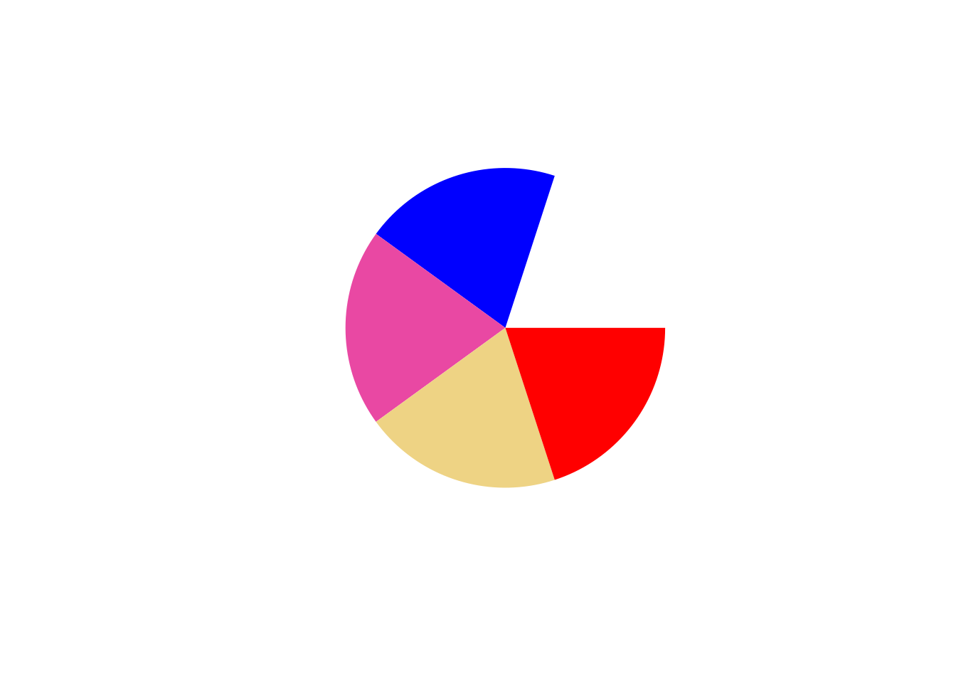
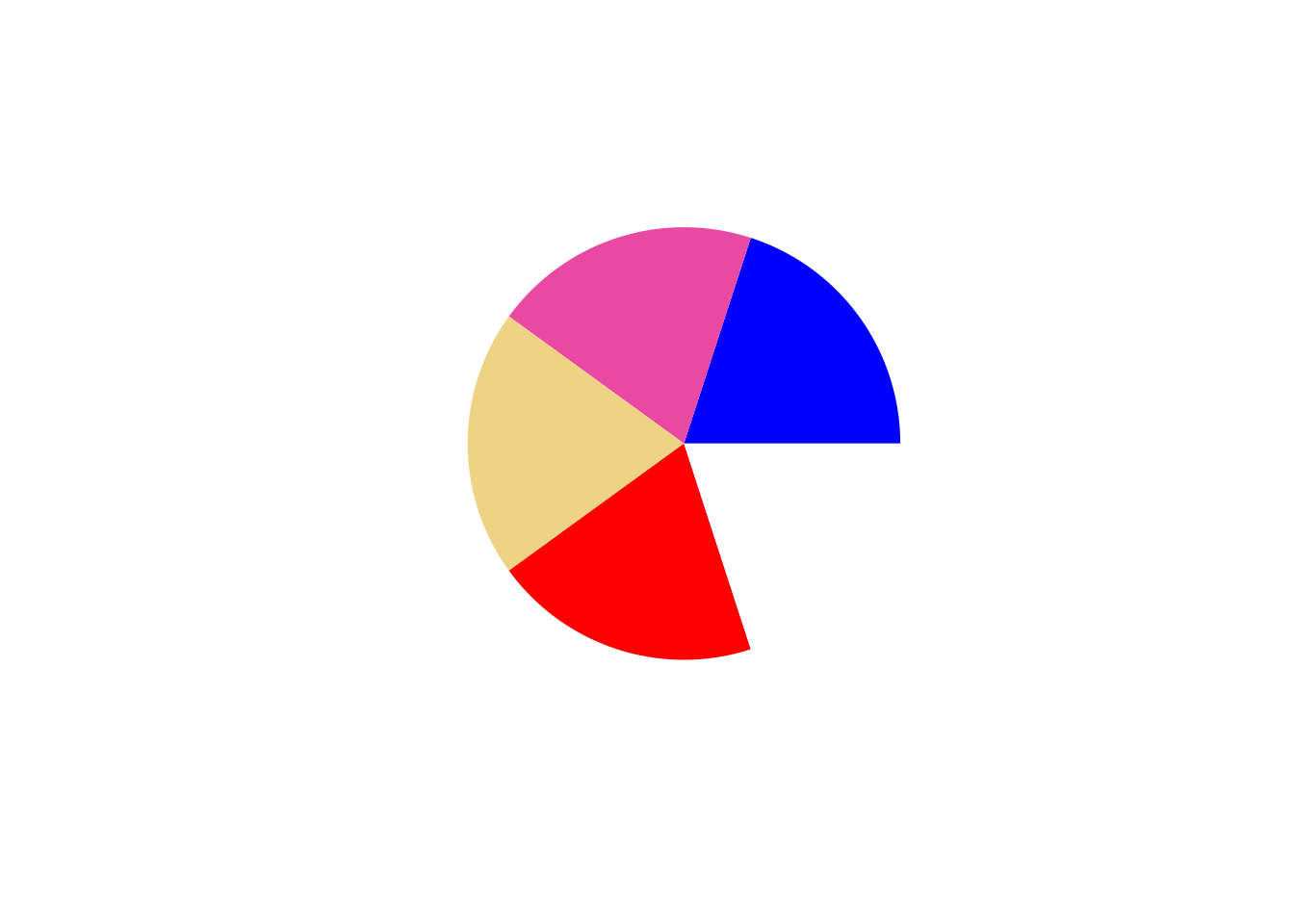
# negative integer inverses the order
c <- colorify(colors = c("red", "white", "blue"), n = 5, order = -1, plot = TRUE)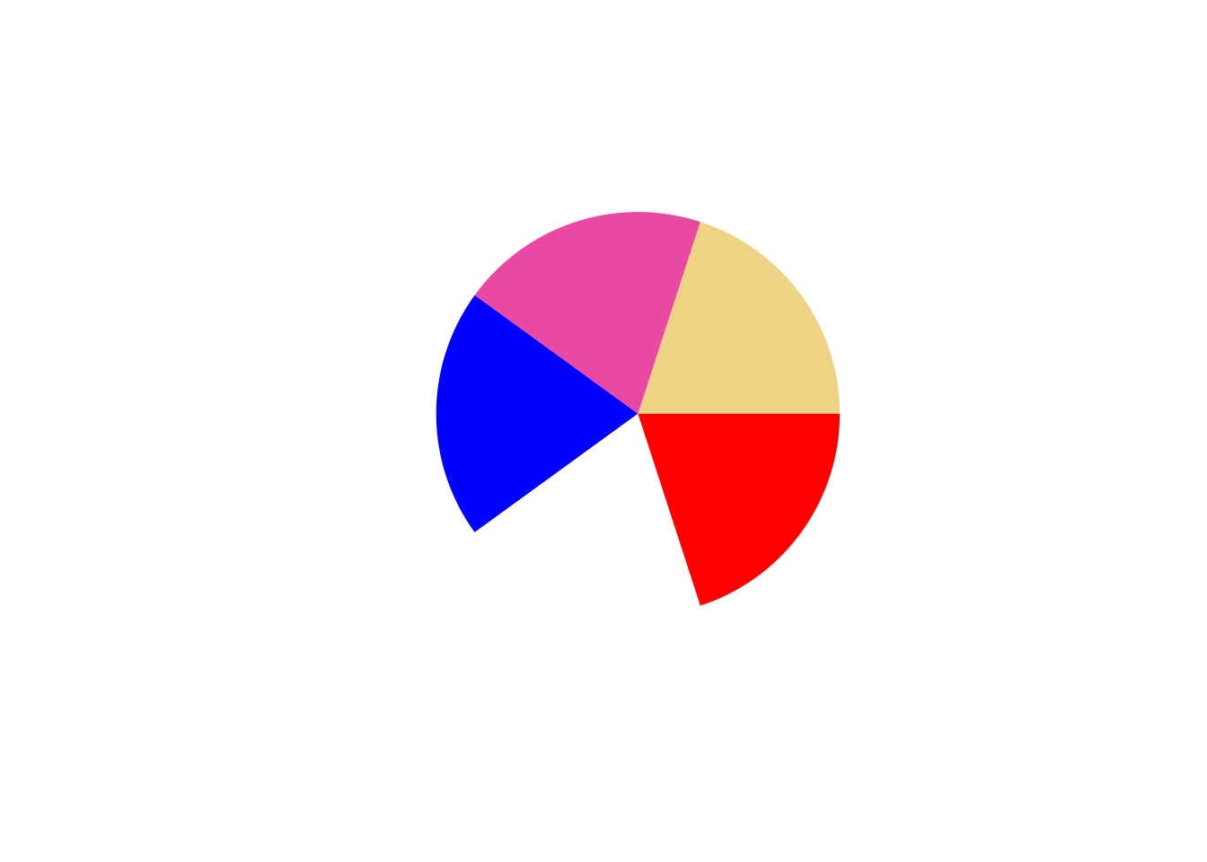
custom palettes
You can supply an available palette in colors, that will be expanded up to requested n.
# note that blue and yellow are cut, as only 10 colors are requested.
c <- colorify(colors = c("Okabe-Ito", "red", "blue", "yellow"), plot = TRUE, n = 10)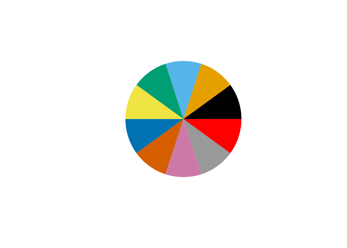

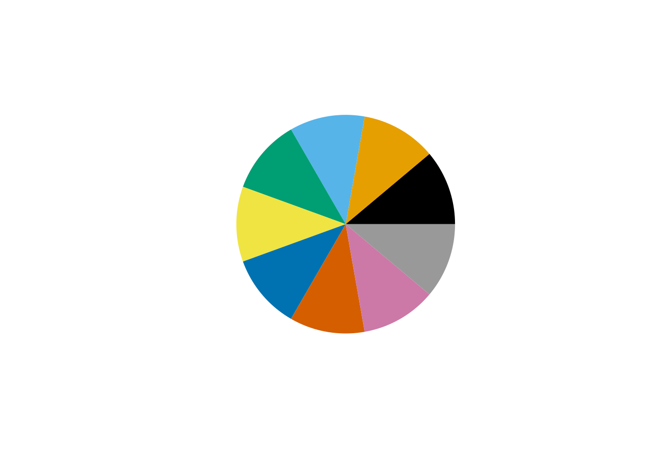
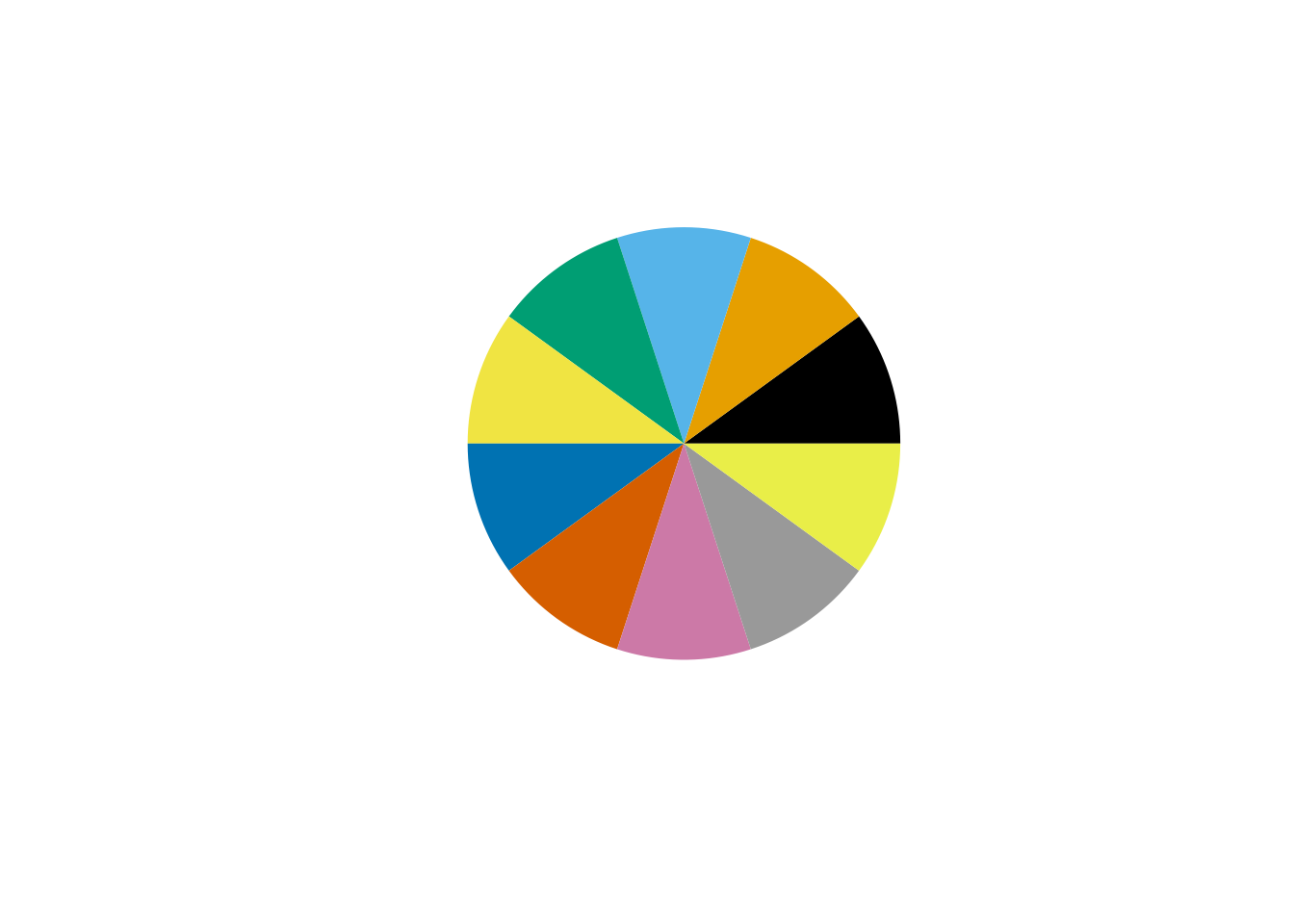
plotting
Plot options, default is circular output, plot = include ‘i’ for image and ‘l’ to plot color index as labels.
g1 <- colorify(colors = c("orange", "red", "white", "blue", "orange"), nn = 15, plot = "l")
g1 <- colorify(colors = c("orange", "red", "white", "blue", "orange"), nn = 15, plot = "i")
g1 <- colorify(colors = c("orange", "red", "white", "blue", "orange"), nn = 15, plot = "il")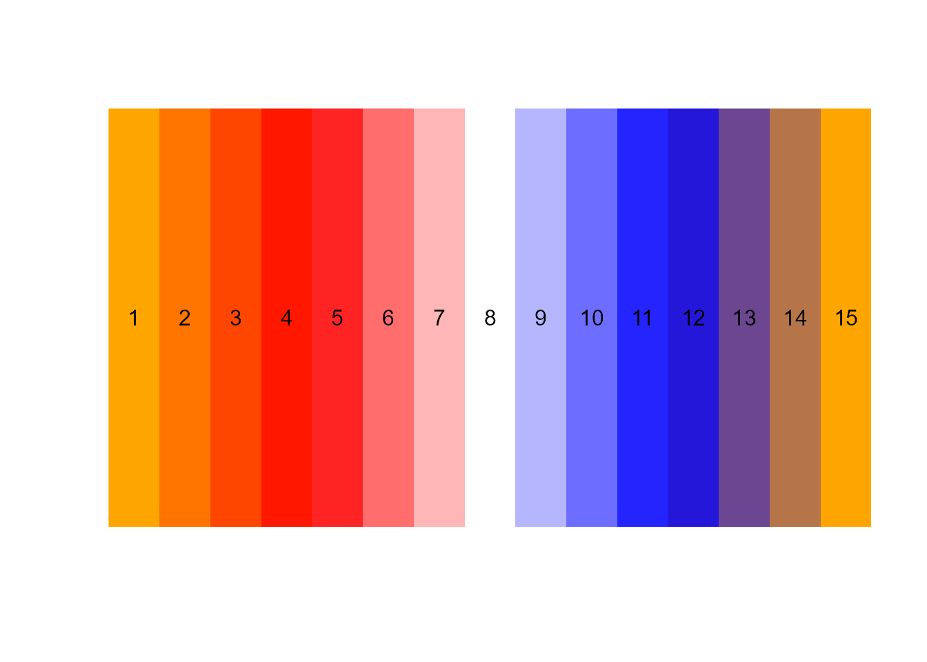
values and factors
Values and factors, let’s say you want your palette to be more or less RGB (red, green, blue)/HSL (hue, saturation, lightness), you can simply tweak their specific channels! Values are intuitively ranged between [0-100] (instead of 0-255). Factors are multiplicative.
The order in which values and factors are called matters, play around with combinations to obtain your ideal custom palettes.
Note that a gradient is made from the ‘n’ parameter here, as some palettes are actually called as functions internally.

# r = red, f = factor: rf = 2 to multiply all red values
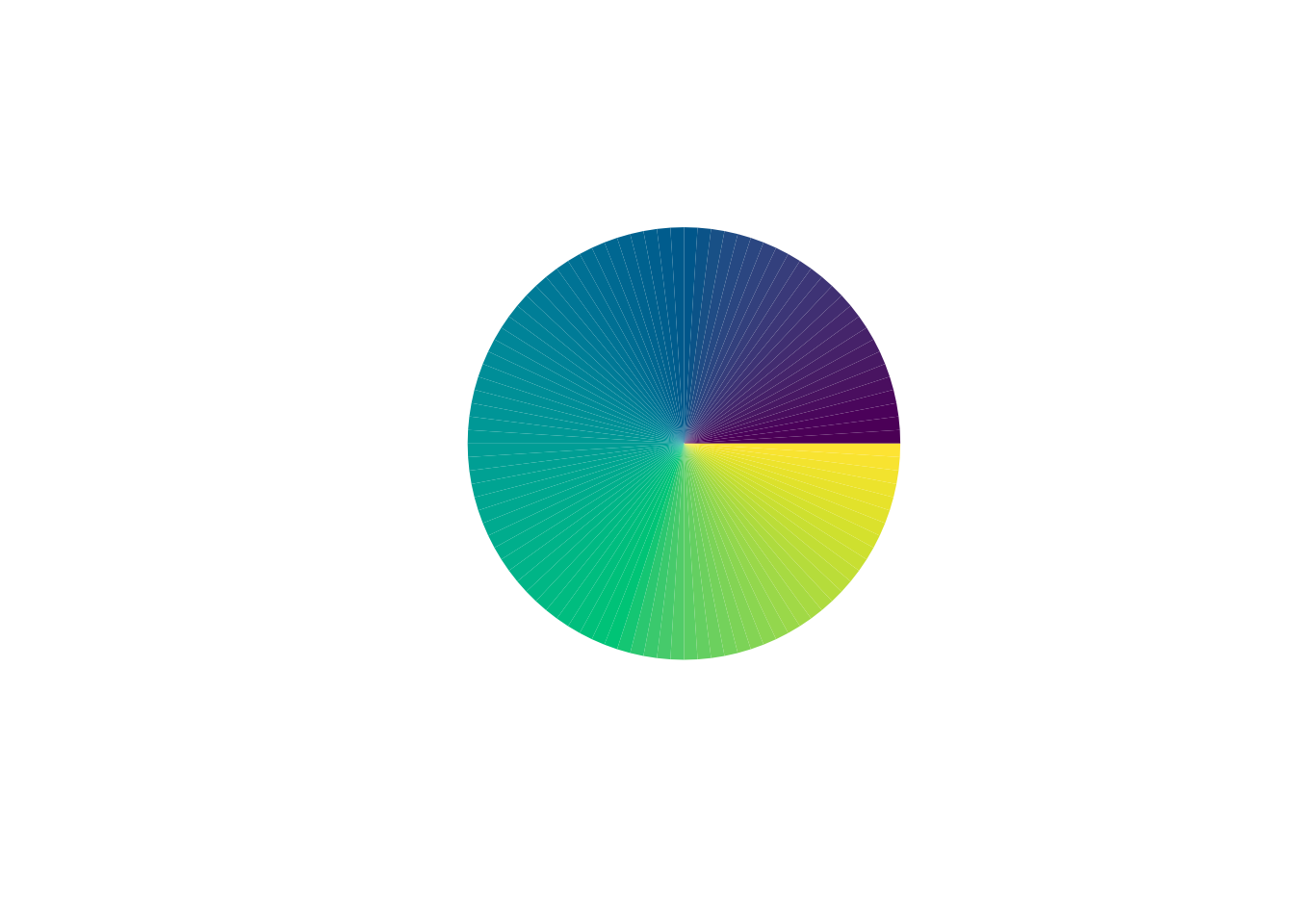
g4 <- colorify(100, colors = c("viridis"), rf = 2, plot = TRUE)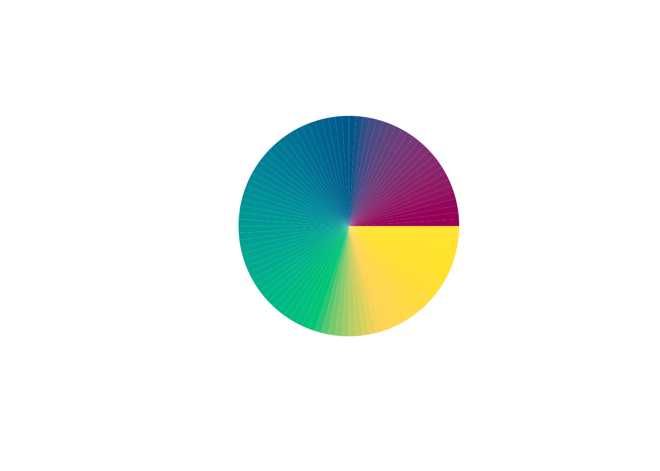
# v = value: rv = 50 to increase all red values by 50, on a scale between 0-100
g5 <- colorify(100, colors = c("viridis"), rv = 50, plot = TRUE)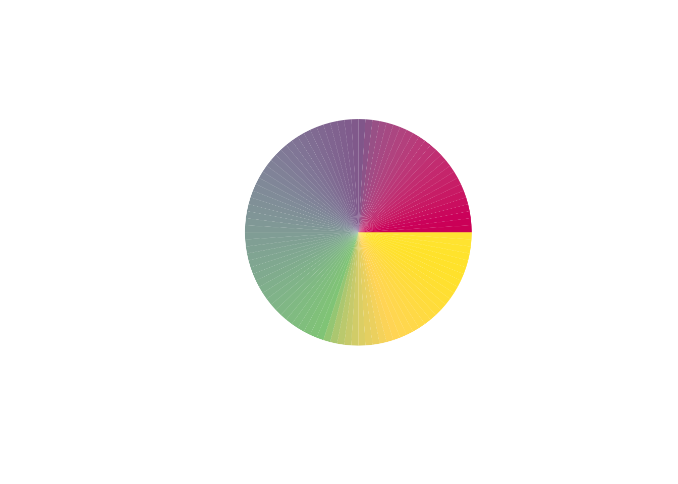
# first, multiply red values by 2, then increase red values by 50
g6 <- colorify(100, colors = c("viridis"), rf = 2, rv = 50, plot = TRUE)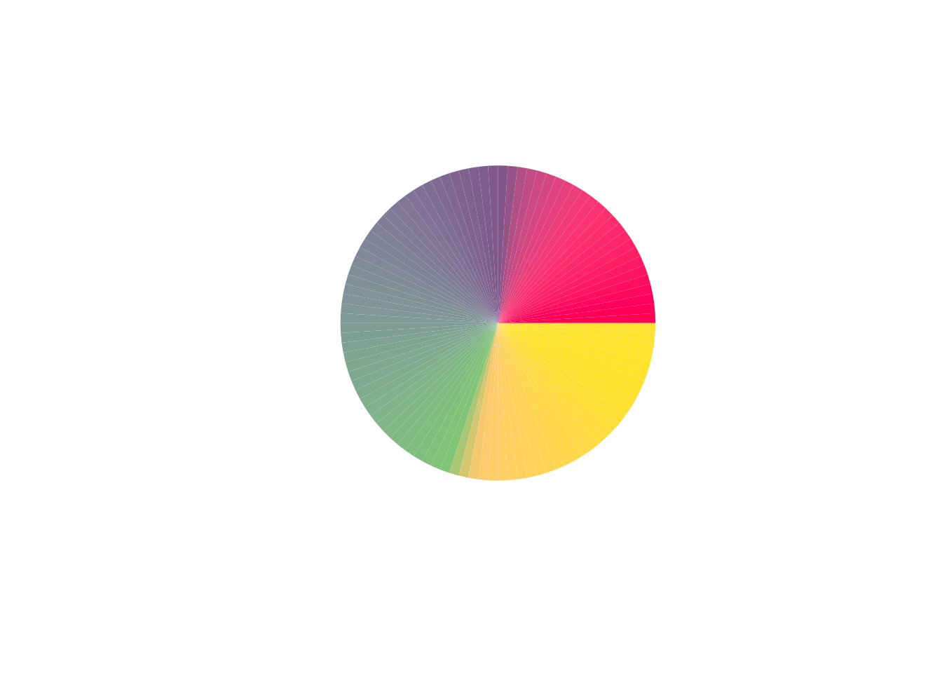
# first, increase red values by 50, then multiply red values by 2
g7 <- colorify(100, colors = c("viridis"), rv = 50, rf = 2, plot = TRUE)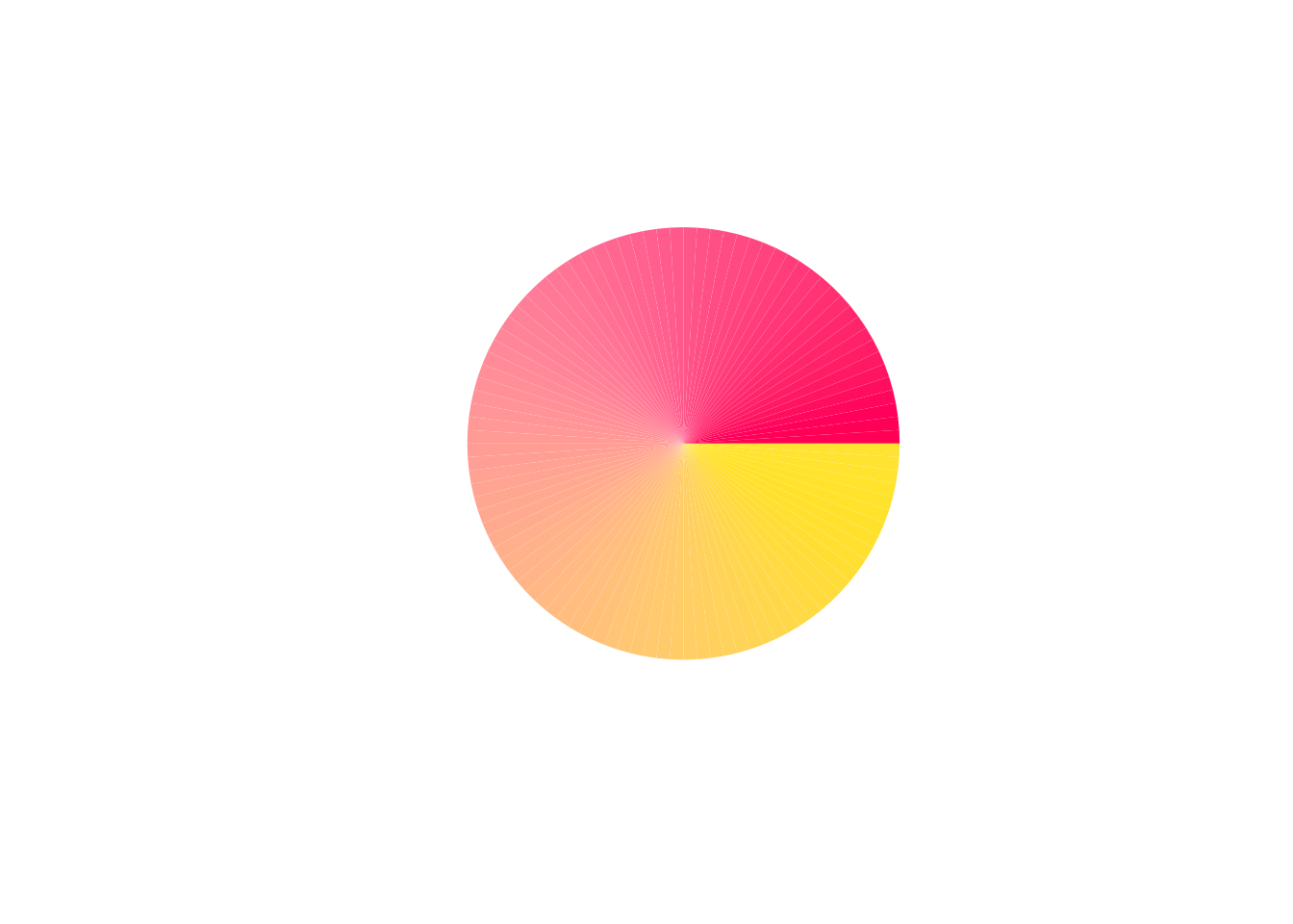
# float factor decrease values by multiplication
g8 <- colorify(100, colors = c("viridis"), bf = .5, plot = TRUE)
# negative values work to decrease values
g9 <- colorify(100, colors = c("viridis"), bv = -100, gv = -50, plot = TRUE)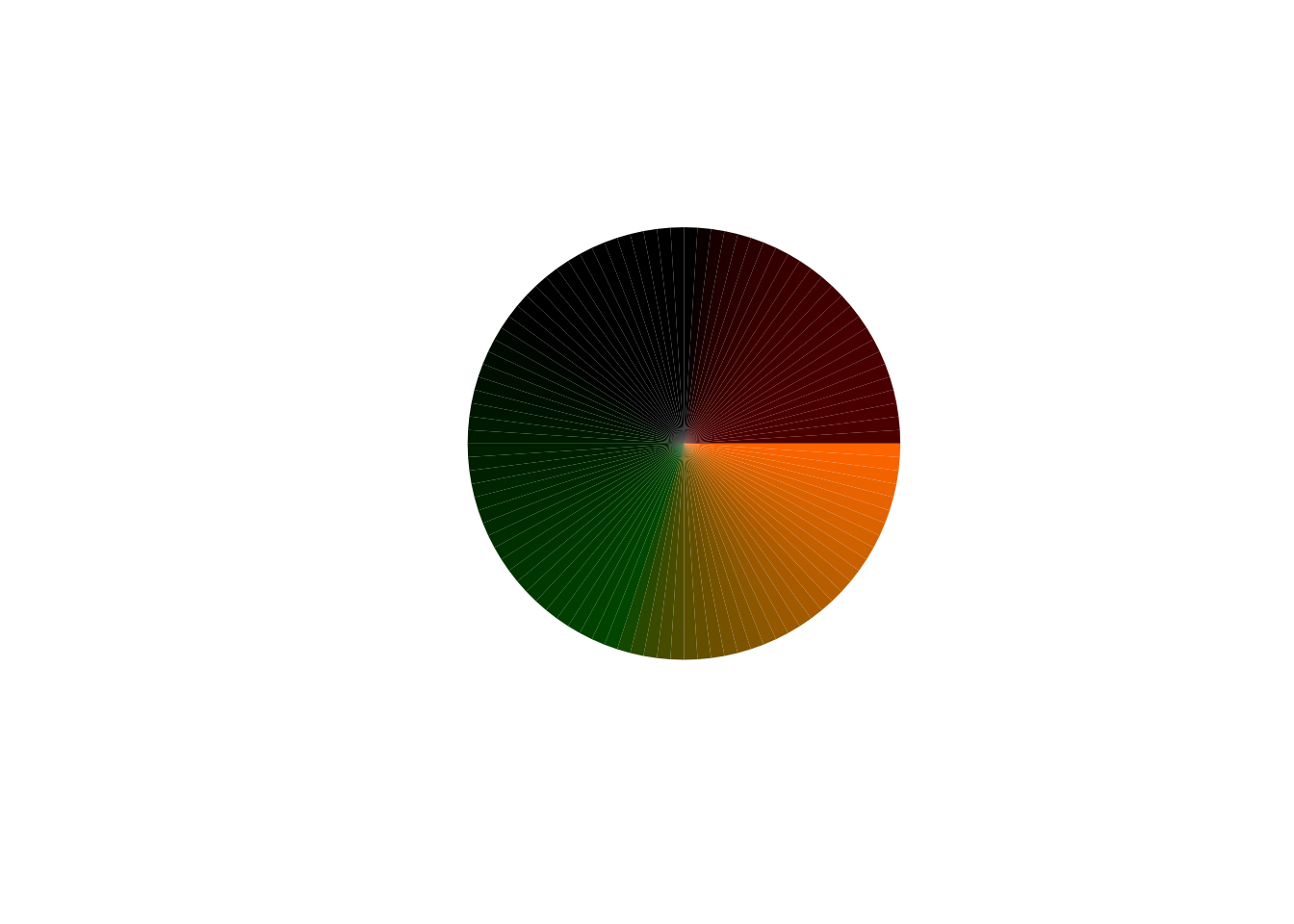
minimum and maximum values
When value and factor adjustments are made, the .min and .max parameters are used to set minimum and maximum RGB/HSL values.

# same factor decrease, yet limited by minimum value
g10 <- colorify(100, colors = c("viridis"), bf = .5, bmin = 40, plot = TRUE)
# need factor/value change to use min/max value
g11 <- colorify(100, colors = c("viridis"), bf = 1, bmax = 40, plot = TRUE)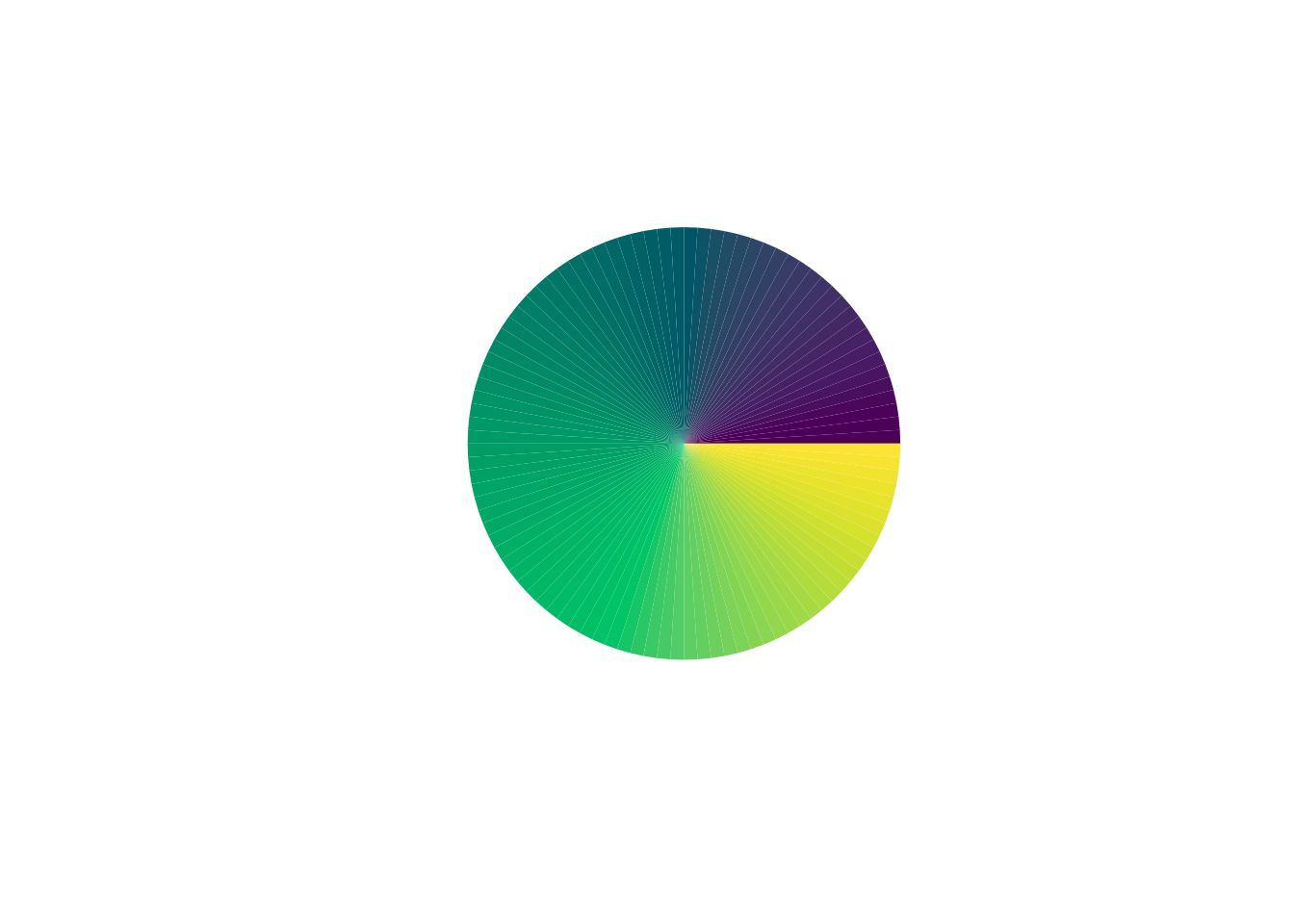
# can use them in combination
g12 <- colorify(100, colors = c("viridis"), bf = 1, bmin = 40, bmax = 40,  plot = TRUE)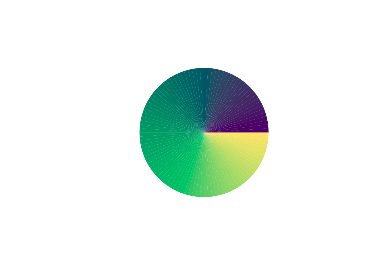
locking
The colors_lock can be used by locking specific colors by numerical index, starting from 1. colors_lock can also be used by patterning, as long as the nn % length of the boolean character == 0. colors_lock can be inversed by putting a ! in front of the given vector.
# lock by index
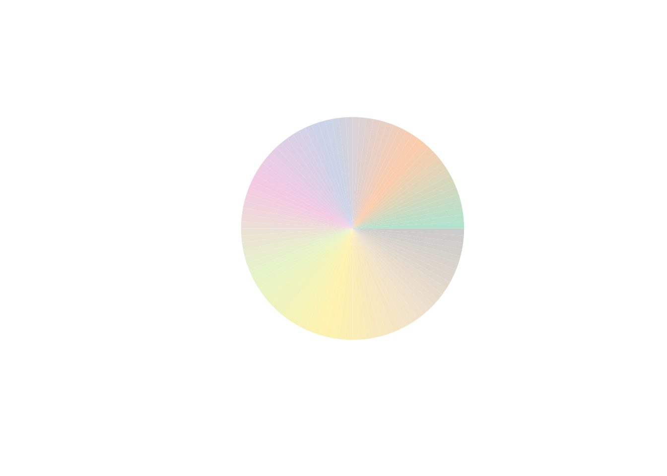
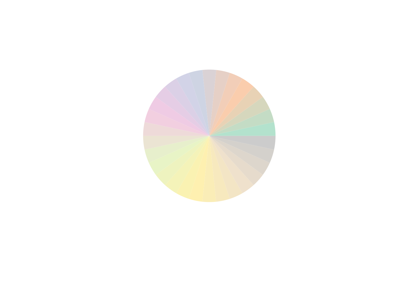
c <- colorify(colors = c("pastel2"), nn = 30, colors_lock = c(4, 5, 6, 10, 11, 12), lf = 0.5, plot = TRUE)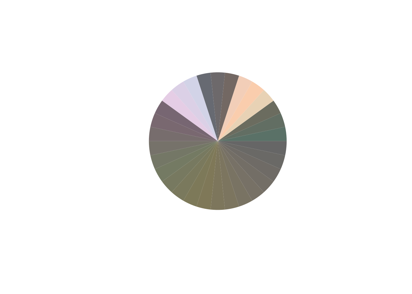
# inverse lock by index
c <- colorify(colors = c("pastel2"), nn = 30, colors_lock = -c(4:12), lf = 0.5, plot = TRUE)
# lock by patterns
c <- colorify(colors = c("pastel2"), nn = 30, colors_lock = c(TRUE, FALSE), lf = 0.5, plot = TRUE)
c <- colorify(colors = c("pastel2"), nn = 30, colors_lock = c(TRUE, FALSE, FALSE), lf = 0.5, plot = TRUE)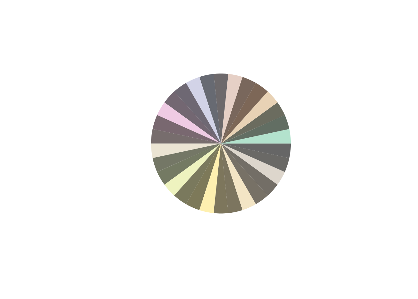
mapping
colors_map takes a vector of values matching the vector of (generated) colors, returning a color_map function which can then be used to generate colors based on supplied values to it.
color_map <- colorify(colors = c("red", "white", "blue"), colors_map = c(0, 500, 1000))
# note the map is then given values to map back to the given color ranges from colors_map
m1 <- colorify(colors = color_map(0:1000), plot = TRUE)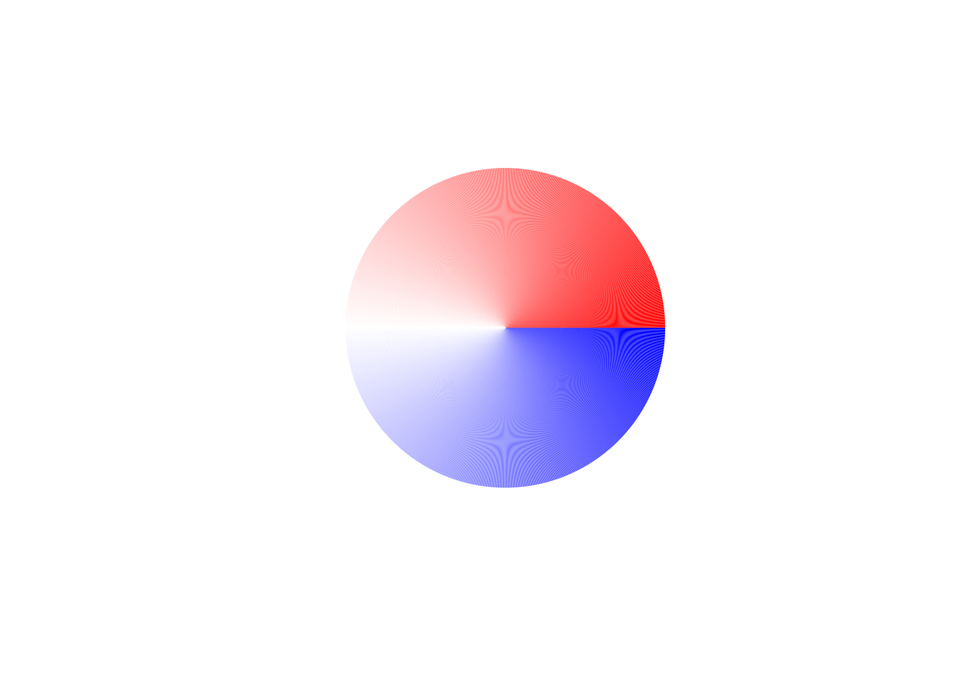
display_palettes()
all palettes
The base use of display_palettes() shows all available palettes in coloRify, that can be used with colorify(colors = c(…)).

#>     Viridis-turbo         grDevices         grDevices         grDevices
#>           "Turbo"         "Rainbow"            "Heat"         "Terrain"
#>         grDevices         grDevices               hcl               hcl
#>            "Topo"              "Cm"        "Pastel 1"          "Dark 2"
#>               hcl               hcl               hcl               hcl
#>          "Dark 3"           "Set 2"           "Set 3"            "Warm"
#>               hcl               hcl               hcl               hcl
#>            "Cold"        "Harmonic"         "Dynamic"           "Grays"
#>               hcl               hcl               hcl               hcl
#>     "Light Grays"         "Blues 2"         "Blues 3"       "Purples 2"
#>               hcl               hcl               hcl               hcl
#>       "Purples 3"          "Reds 2"          "Reds 3"        "Greens 2"
#>               hcl               hcl               hcl               hcl
#>        "Greens 3"            "Oslo"     "Purple-Blue"      "Red-Purple"
#>               hcl               hcl               hcl               hcl
#>        "Red-Blue"   "Purple-Orange"   "Purple-Yellow"     "Blue-Yellow"
#>               hcl               hcl               hcl               hcl
#>    "Green-Yellow"      "Red-Yellow"            "Heat"          "Heat 2"
#>               hcl               hcl               hcl               hcl
#>         "Terrain"       "Terrain 2"         "Viridis"          "Plasma"
#>               hcl               hcl               hcl               hcl
#>         "Inferno"          "Rocket"            "Mako"       "Dark Mint"
#>               hcl               hcl               hcl               hcl
#>            "Mint"          "BluGrn"            "Teal"         "TealGrn"
#>               hcl               hcl               hcl               hcl
#>           "Emrld"           "BluYl"        "ag_GrnYl"           "Peach"
#>               hcl               hcl               hcl               hcl
#>          "PinkYl"            "Burg"          "BurgYl"           "RedOr"
#>               hcl               hcl               hcl               hcl
#>           "OrYel"            "Purp"          "PurpOr"          "Sunset"
#>               hcl               hcl               hcl               hcl
#>         "Magenta"      "SunsetDark"       "ag_Sunset"          "BrwnYl"
#>               hcl               hcl               hcl               hcl
#>          "YlOrRd"          "YlOrBr"            "OrRd"         "Oranges"
#>               hcl               hcl               hcl               hcl
#>            "YlGn"          "YlGnBu"            "Reds"            "RdPu"
#>               hcl               hcl               hcl               hcl
#>            "PuRd"         "Purples"          "PuBuGn"            "PuBu"
#>               hcl               hcl               hcl               hcl
#>          "Greens"            "BuGn"            "GnBu"            "BuPu"
#>               hcl               hcl               hcl               hcl
#>           "Blues"         "Lajolla"           "Turku"          "Hawaii"
#>               hcl               hcl               hcl               hcl
#>          "Batlow"        "Blue-Red"      "Blue-Red 2"      "Blue-Red 3"
#>               hcl               hcl               hcl               hcl
#>       "Red-Green"    "Purple-Green"    "Purple-Brown"     "Green-Brown"
#>               hcl               hcl               hcl               hcl
#>   "Blue-Yellow 2"   "Blue-Yellow 3"    "Green-Orange"    "Cyan-Magenta"
#>               hcl               hcl               hcl               hcl
#>          "Tropic"            "Broc"            "Cork"             "Vik"
#>               hcl               hcl               hcl               hcl
#>          "Berlin"          "Lisbon"          "Tofino"        "ArmyRose"
#>               hcl               hcl               hcl               hcl
#>           "Earth"            "Fall"          "Geyser"        "TealRose"
#>               hcl               hcl               hcl               hcl
#>           "Temps"            "PuOr"            "RdBu"            "RdGy"
#>               hcl               hcl               hcl               hcl
#>            "PiYG"            "PRGn"            "BrBG"          "RdYlBu"
#>               hcl               hcl               hcl               hcl
#>          "RdYlGn"        "Spectral"        "Zissou 1"         "Cividis"
#>               hcl               pal               pal               pal
#>            "Roma"              "R3"              "R4"         "ggplot2"
#>               pal               pal               pal               pal
#>       "Okabe-Ito"          "Accent"          "Dark 2"          "Paired"
#>               pal               pal               pal               pal
#>        "Pastel 1"        "Pastel 2"           "Set 1"           "Set 2"
#>               pal               pal               pal               pal
#>           "Set 3"      "Tableau 10" "Classic Tableau"   "Polychrome 36"
#>               pal
#>        "Alphabet"
n palettes
The n parameter here is used to show the amount of colors per palette.
p1 <- display_palettes(10)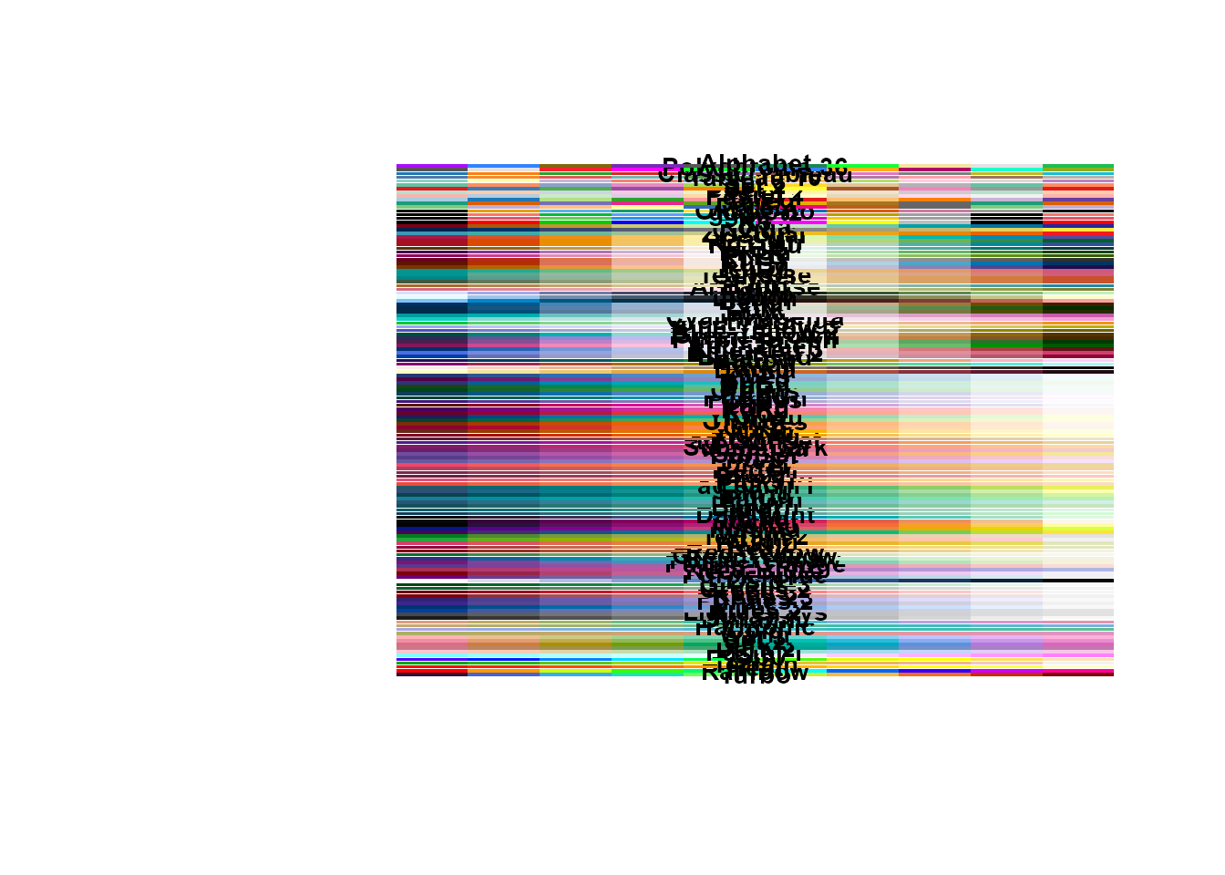
# display 100 colors per palette
p2 <- display_palettes(100)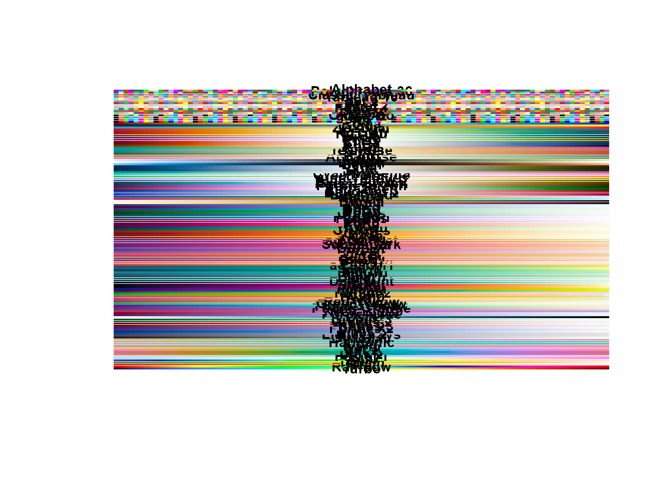
palettes by index
The i_palettes parameter can also be passed numeric integers to get a more clear palette view.
# display palettes by index
display_palettes(i_palettes = 50:75)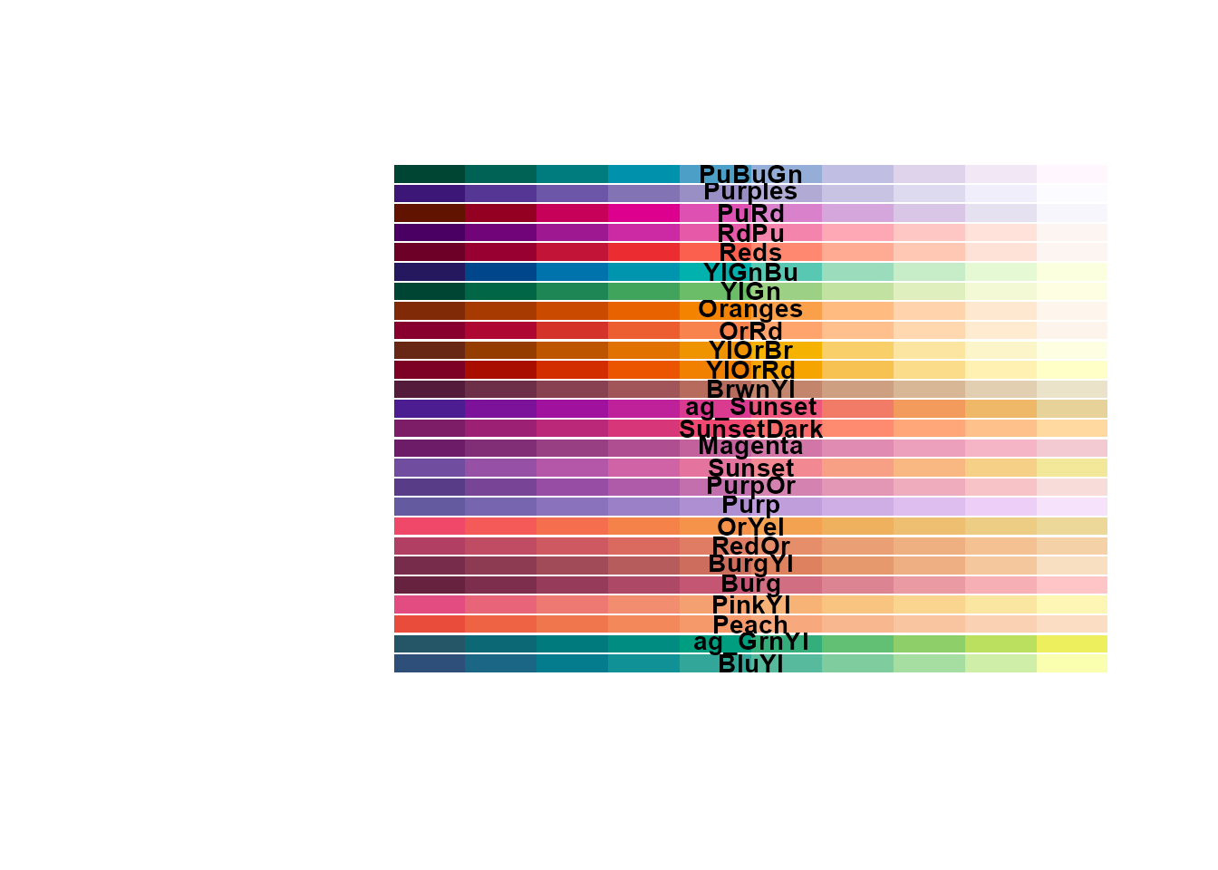
#>          hcl          hcl          hcl          hcl          hcl          hcl
#>      "BluYl"   "ag_GrnYl"      "Peach"     "PinkYl"       "Burg"     "BurgYl"
#>          hcl          hcl          hcl          hcl          hcl          hcl
#>      "RedOr"      "OrYel"       "Purp"     "PurpOr"     "Sunset"    "Magenta"
#>          hcl          hcl          hcl          hcl          hcl          hcl
#> "SunsetDark"  "ag_Sunset"     "BrwnYl"     "YlOrRd"     "YlOrBr"       "OrRd"
#>          hcl          hcl          hcl          hcl          hcl          hcl
#>    "Oranges"       "YlGn"     "YlGnBu"       "Reds"       "RdPu"       "PuRd"
#>          hcl          hcl
#>    "Purples"     "PuBuGn"
display_palettes(i_palettes = c(1, 5, 10, 20, 40, 100, 119))
#> Viridis-turbo     grDevices           hcl           hcl           hcl
#>       "Turbo"        "Topo"       "Set 2"   "Purples 2"      "Plasma"
#>           hcl           hcl
#>         "Vik"    "Zissou 1"
popular palettes
Popular palettes from commonly used color packages are available.
display_palettes(10, "rcolorbrewer")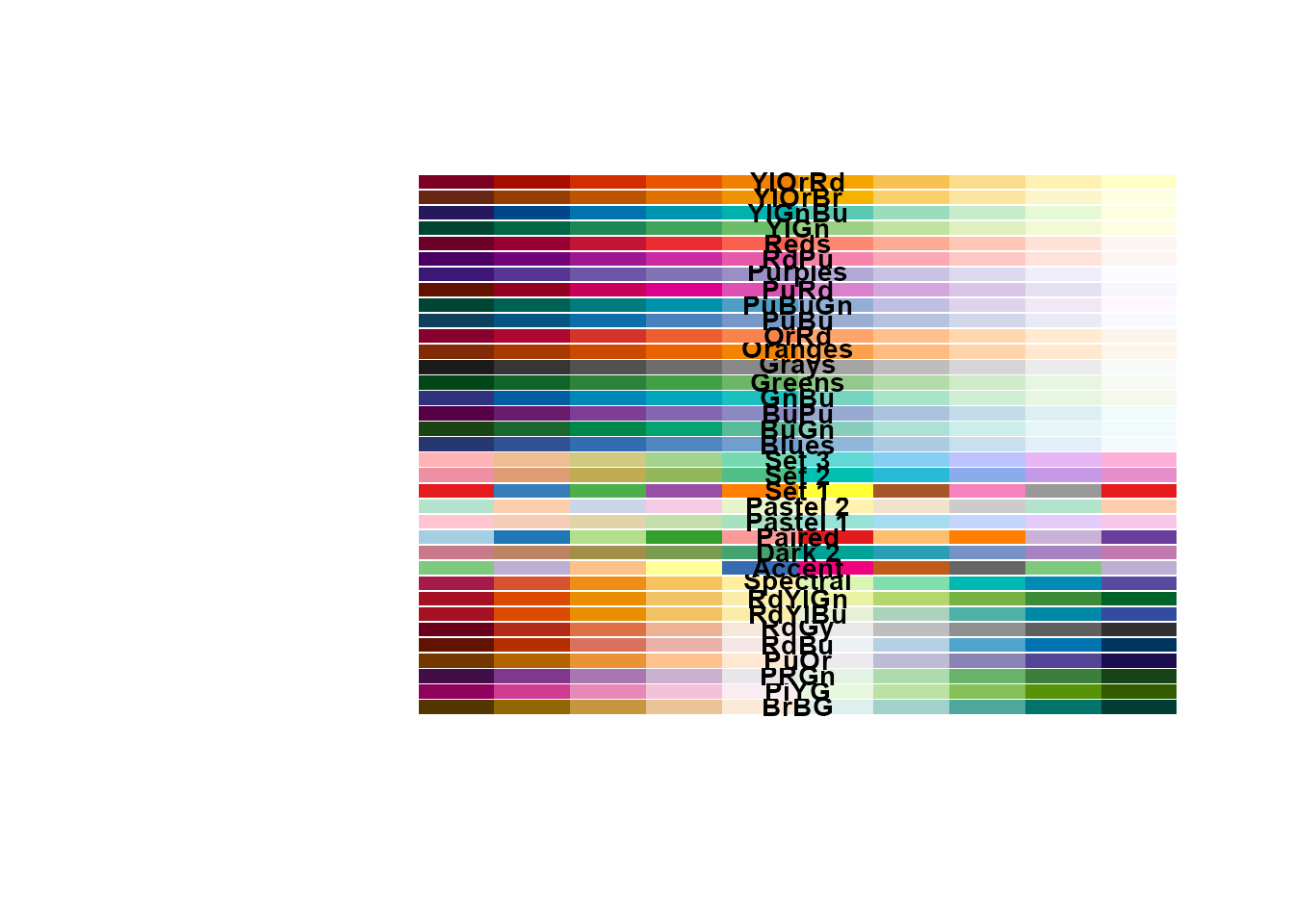
#>        hcl        hcl        hcl        hcl        hcl        hcl        hcl
#>     "BrBG"     "PiYG"     "PRGn"     "PuOr"     "RdBu"     "RdGy"   "RdYlBu"
#>        hcl        hcl        pal        hcl        pal        hcl        pal
#>   "RdYlGn" "Spectral"   "Accent"   "Dark 2"   "Paired" "Pastel 1" "Pastel 2"
#>        pal        hcl        hcl        hcl        hcl        hcl        hcl
#>    "Set 1"    "Set 2"    "Set 3"    "Blues"     "BuGn"     "BuPu"     "GnBu"
#>        hcl        hcl        hcl        hcl        hcl        hcl        hcl
#>   "Greens"    "Grays"  "Oranges"     "OrRd"     "PuBu"   "PuBuGn"     "PuRd"
#>        hcl        hcl        hcl        hcl        hcl        hcl        hcl
#>  "Purples"     "RdPu"     "Reds"     "YlGn"   "YlGnBu"   "YlOrBr"   "YlOrRd"
display_palettes(10, "viridis")
#>           hcl           hcl           hcl           hcl           hcl
#>     "Viridis"      "Plasma"     "Inferno"     "Cividis"      "Rocket"
#>           hcl Viridis-turbo
#>        "Mako"       "Turbo"
display_palettes(10, "rainbow") # grDevices palettes
#> grDevices grDevices grDevices grDevices grDevices
#> "Rainbow"    "Heat" "Terrain"    "Topo"      "Cm"
bordered palettes
Visualize palettes with borders around individual colors.
display_palettes(n = 10, i_palettes = 1:10, border = TRUE)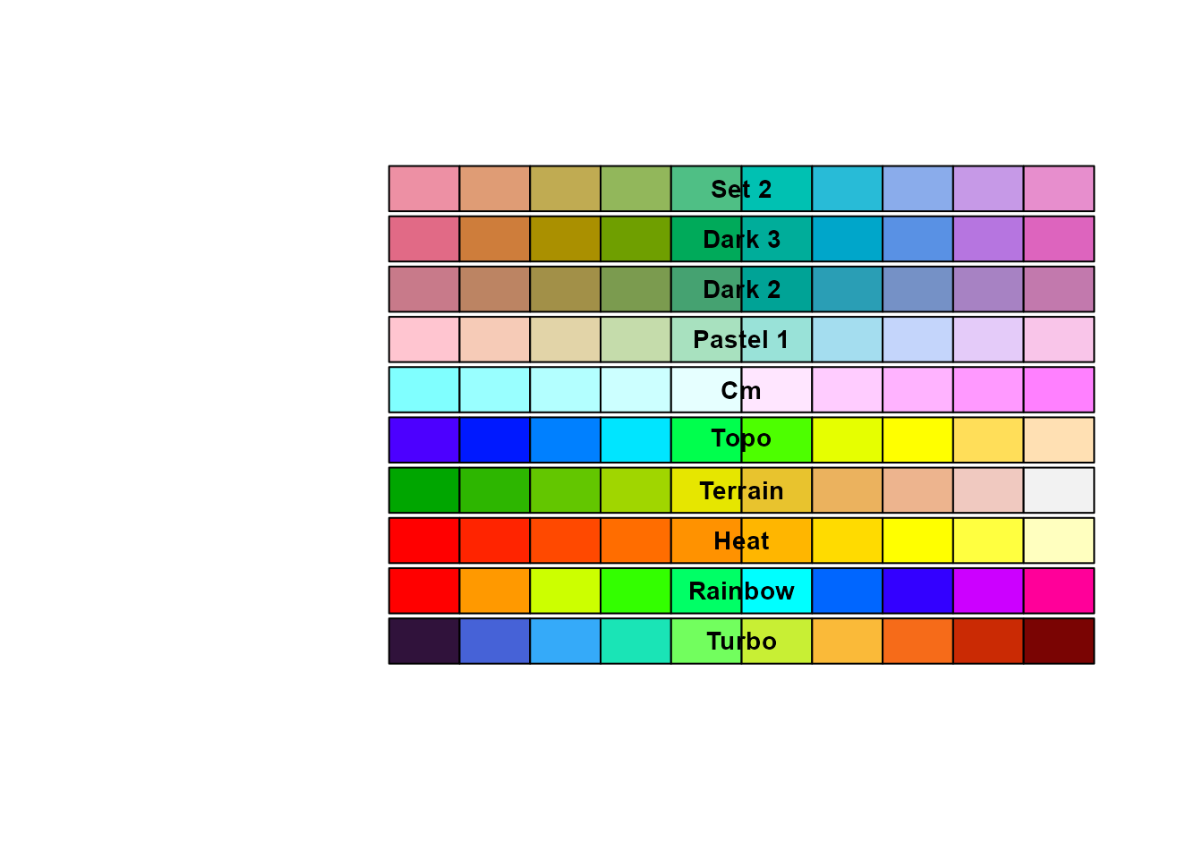
#> Viridis-turbo     grDevices     grDevices     grDevices     grDevices
#>       "Turbo"     "Rainbow"        "Heat"     "Terrain"        "Topo"
#>     grDevices           hcl           hcl           hcl           hcl
#>          "Cm"    "Pastel 1"      "Dark 2"      "Dark 3"       "Set 2"
ggplot2 bindings
These functions are bindings similar to the ggplot2 scale_* functions, to use them ggplot2 has to be installed and loaded.
install.packages("ggplot2")
library(ggplot2)
scale_color_colorify()
non-discrete
dsub <- subset(ggplot2::diamonds, x > 5 & x < 6 & y > 5 & y < 6)
dsub$diff <- with(dsub, sqrt(abs(x - y)) * sign(x - y))

ggplot2::ggplot(dsub, ggplot2::aes(x, y, colour = diff)) +
  ggplot2::geom_point() +
  scale_color_colorify(n = 4, colors = "viridis") +
  ggplot2::theme_bw()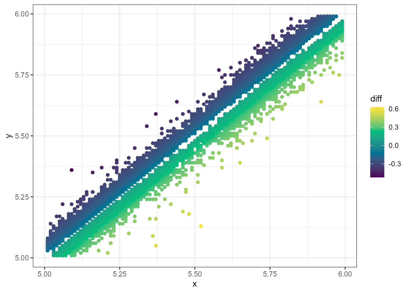
discrete
p <- ggplot2::ggplot(mtcars, ggplot2::aes(wt, mpg))

p + ggplot2::geom_point(size = 4, ggplot2::aes(colour = factor(cyl))) +
  ggplot2::theme_bw() +
  scale_color_colorify(discrete = TRUE, colors = c("red", "blue", "yellow"))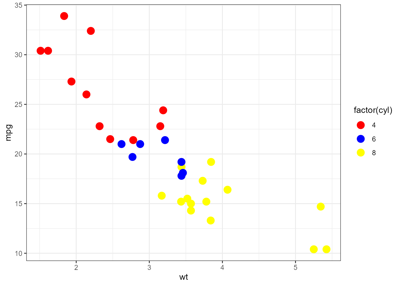
scale_fill_colorify()
non-discrete
dat <- data.frame(x = rnorm(10000), y = rnorm(10000))

ggplot2::ggplot(dat, ggplot2::aes(x = x, y = y)) +
  ggplot2::geom_hex() + ggplot2::coord_fixed() +
  scale_fill_colorify(colors = "viridis", n = 4) + ggplot2::theme_bw()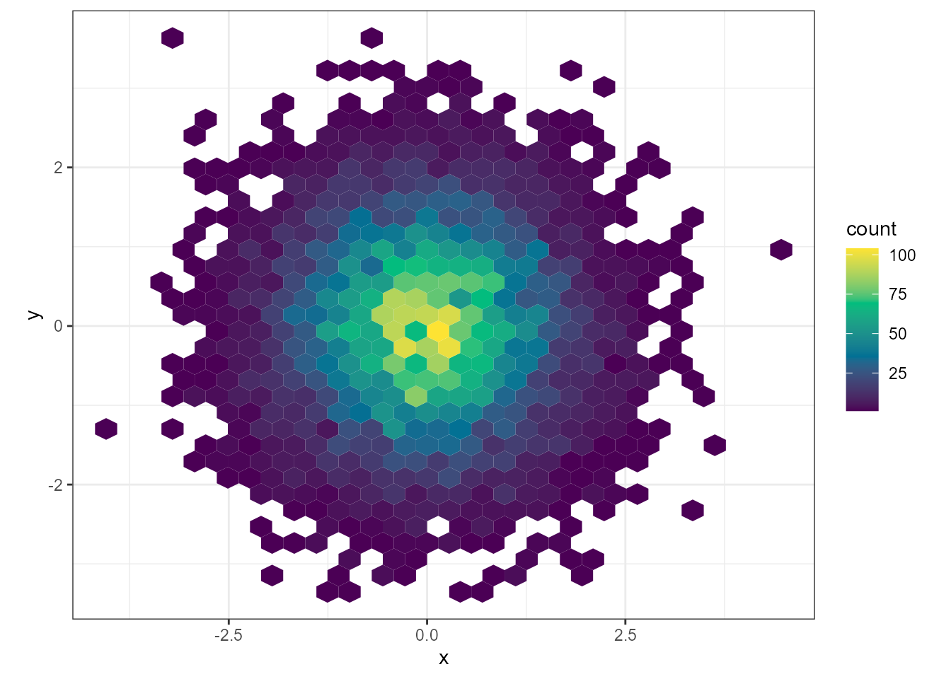
discrete
df <- data.frame(category = c("A", "B", "C", "D"), value = c(10, 23, 15, 8))

ggplot2::ggplot(df, ggplot2::aes(x = category, y = value, fill = category)) +
  ggplot2::geom_bar(stat = "identity") +
  scale_fill_colorify(discrete = TRUE, colors = "viridis")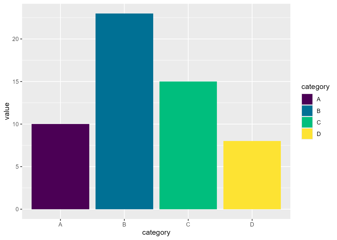
colortistry()
My colorful monstrosity I contribute to the #Rtistry community! I heartily welcome creative contributions using coloRify <3
colors_list <- list()
for (i in seq(100)) {
  colors_list[[i]] <- colorify(n = 100, colors = "rainbow", colors_lock = rep(c(TRUE, FALSE, FALSE, FALSE, FALSE), 20), hf = 25 / i, lf = i / 20)
  if (i %% 3) colors_list[[i]] <- colorify(n = 100, colors = "rainbow", colors_lock = rep(c(FALSE, FALSE, TRUE, FALSE, FALSE), 20), hf = 30 / i, lf = i / 20)
  if (i %% 4) colors_list[[i]] <- colorify(n = 100, colors = "rainbow", colors_lock = rep(c(FALSE, FALSE, FALSE, TRUE, FALSE), 20), hf = 50 / i, lf = i / 40)
  if (i %% 5) colors_list[[i]] <- colorify(n = 100, colors = "rainbow", colors_lock = rep(c(FALSE, TRUE, FALSE, FALSE, FALSE), 20), hf = 50 / i, sf = i / 50)
}
colortistry(colors_list)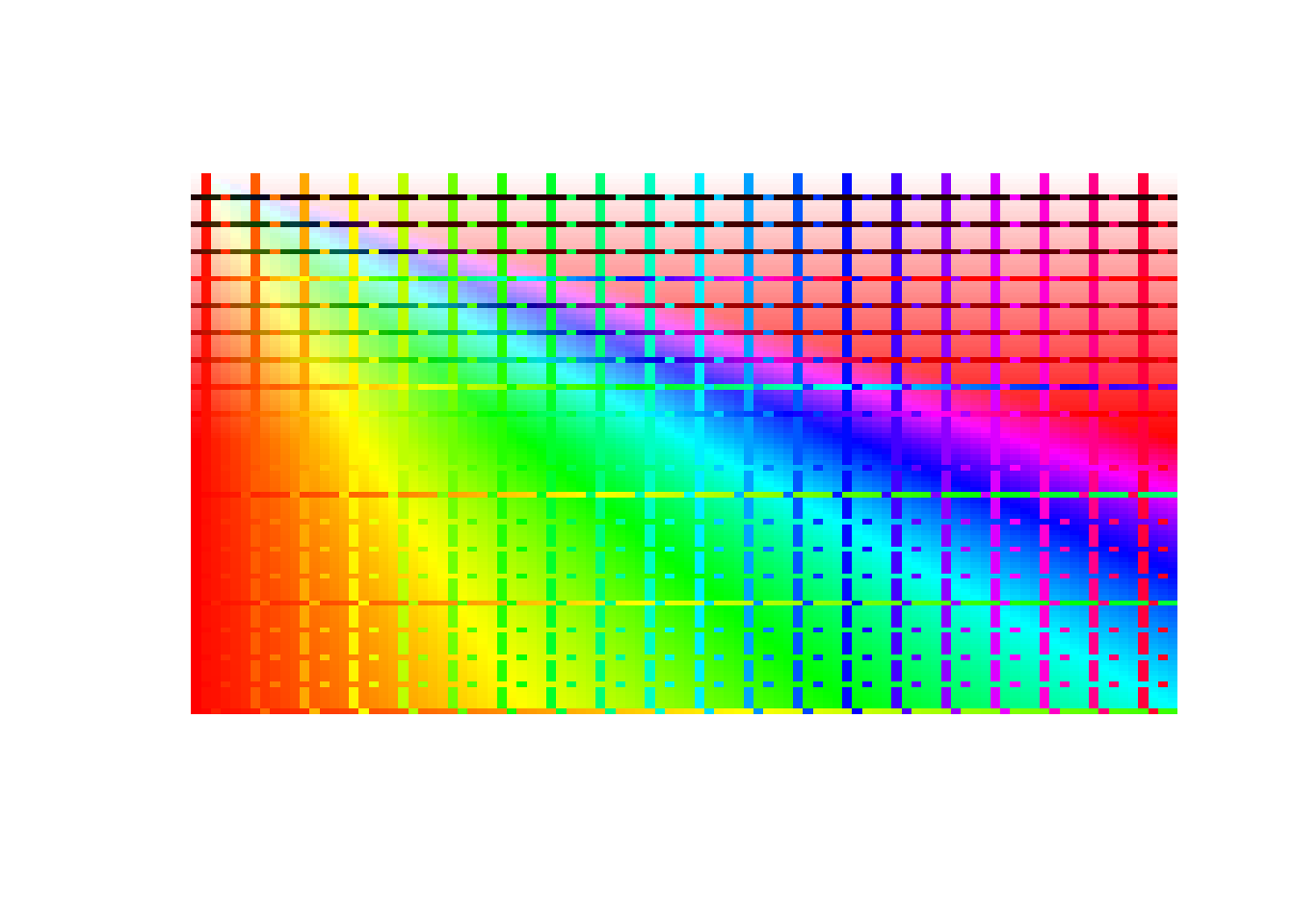
# and with borders
colortistry(colors_list, border_color = "black")
Information
A thank you for your time and effort in using coloRify, I hope it may aid you in COOLORing your visualizations!
Contact
Colorify was developed by Maurits Unkel at the Erasmus Medical Center in the department of Psychiatry. Source code is available through GitHub: https://github.com/mauritsunkel/colorify Questions regarding coloRify can be sent to: mauritsunkel@gmail.com
Issues and contributions
For issues and contributions, please find the coloRify Github page: https://github.com/mauritsunkel/colorify/issues
FAQ
Q: How can I easily test my coloRify palettes on actual visualizations?
- A: I advise you to use colorspace::demoplot(colorify(5), type = “heatmap”), switching up type for specific plot types and replacing the colorify() call with your own.
Session info
sessionInfo()
#> R version 4.6.0 (2026-04-24)
#> Platform: x86_64-pc-linux-gnu
#> Running under: Ubuntu 24.04.4 LTS
#>
#> Matrix products: default
#> BLAS:   /usr/lib/x86_64-linux-gnu/openblas-pthread/libblas.so.3
#> LAPACK: /usr/lib/x86_64-linux-gnu/openblas-pthread/libopenblasp-r0.3.26.so;  LAPACK version 3.12.0
#>
#> locale:
#>  [1] LC_CTYPE=C.UTF-8       LC_NUMERIC=C           LC_TIME=C.UTF-8
#>  [4] LC_COLLATE=C.UTF-8     LC_MONETARY=C.UTF-8    LC_MESSAGES=C.UTF-8
#>  [7] LC_PAPER=C.UTF-8       LC_NAME=C              LC_ADDRESS=C
#> [10] LC_TELEPHONE=C         LC_MEASUREMENT=C.UTF-8 LC_IDENTIFICATION=C
#>
#> time zone: UTC
#> tzcode source: system (glibc)
#>
#> attached base packages:
#> [1] stats     graphics  grDevices utils     datasets  methods   base
#>
#> other attached packages:
#> [1] colorify_1.0.0
#>
#> loaded via a namespace (and not attached):
#>  [1] vctrs_0.7.3        cli_3.6.6          knitr_1.51         rlang_1.2.0
#>  [5] xfun_0.58          otel_0.2.0         S7_0.2.2           textshaping_1.0.5
#>  [9] jsonlite_2.0.0     labeling_0.4.3     glue_1.8.1         htmltools_0.5.9
#> [13] ragg_1.5.2         sass_0.4.10        scales_1.4.0       rmarkdown_2.31
#> [17] grid_4.6.0         evaluate_1.0.5     jquerylib_0.1.4    fastmap_1.2.0
#> [21] yaml_2.3.12        lifecycle_1.0.5    compiler_4.6.0     RColorBrewer_1.1-3
#> [25] fs_2.1.0           farver_2.1.2       systemfonts_1.3.2  digest_0.6.39
#> [29] R6_2.6.1           bslib_0.11.0       withr_3.0.2        tools_4.6.0
#> [33] gtable_0.3.6       pkgdown_2.2.0      ggplot2_4.0.3      cachem_1.1.0
#> [37] desc_1.4.3